


Hello World!
I'm really excited to write my very first article.
We will be talking about and also building a Linear Classification algorithm with Tensorflow 2.0. Tensorflow is arguably the most popular framework for machine learning and deep learning with Pytorch usually coming in second. There will be future posts about Pytorch when I'm done with this Tensorflow series.
TensorFlow is an end-to-end open-source platform for machine learning. It has a comprehensive, flexible ecosystem of tools, libraries and community resources that lets researchers push the state-of-the-art in ML and developers easily build and deploy ML-powered applications.
The codes are written as Jupyter notebooks and run directly in Google Colab—a hosted notebook environment that requires no setup.
Refer to this post on how to use Colab
Overview
This is the first part of the mini-series where I will be talking about ANNs, CNNs, RNNs, NLP, RL and how to deploy your models with Tensorflow.
This post assumes you have basic knowledge on how to use the Scikit-learn API, pandas and Numpy.
Linear Classification Theory
Wiki says the goal of classification is to use an object's characteristics to identify which class (or group) it belongs to. A linear classifier achieves this by making a classification decision based on the value of a linear combination of the characteristics. An object's characteristics are also known as feature values and are typically presented to the machine in a vector called a feature vector. The definition is good... but I think things tend to be more understandable when using analogies.
Now imagine you have been given a task to identify albinos. Things you'd normally lookout for are skin colour, hair colour, fiery eyes and maybe dark moles. Those are the features. Assigning albino/not albino is called the label/target. This is a very basic form classification - trying to sort data into two specified values. This is called Binary Classification. Note that there is also a term called Multiclass Classification which refers to those classification tasks that have more than two class labels but still have a specific range of labels.
The Dataset
For this example, we will be using UCI Repository Heart Disease Dataset. The dataset contains 76 attributes, but all published experiments refer to using a subset of 14 of them.
Model Architecture
Note that I will not be going into the maths behind functions. Thankfully, Tensorflow implements the maths for us. For my curious readers, resources will be posted below.
Model architectures originate from a combination of layers with the previous layer learning from the last layer. Since we are building a simple model, we will be using 2 layers: the input layer and the output layer. The first layer is the input and the last layer is the output. If there is more than one hidden layer, we call them “deep” neural networks (Usage and explanation of this in a later post). The model trains by assigning random weights to each data point and uses a cost/loss/error function to calculate the loss or how well the model is performing (The more incorrect our predictions are, the higher the loss function). It then applies gradient descent to minimise the loss. Training is an iterative process and what we want is for the loss per iteration to decrease. We will be visualising this later to ensure that our loss decreases.
Ladies and Gentlemen, shall we...
Note that the parameters set in this code are not particularly the best parameters. They are just the ones that work best for me.
There are no optimal parameters in machine learning, you want to try everything and select what works best for you
Since we are writing in Google colab, we want to first mount our Google drive so as to access the files.
# Load the Drive helper and mount
from google.colab import drive

# This will prompt for authorization.
drive.mount('/content/drive')
Then we import the required libraries
import pandas as pd
import numpy as np
import matplotlib.pyplot as plt
import tensorflow as tf
print(tf.__version__)

>  2.3.0
Next, we want to load in our data and check if we need to apply any preprocessing techniques.
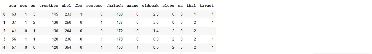
data = pd.read_csv('/content/drive/My Drive/Tensorflow/heart.csv')
data.head()
data.info()
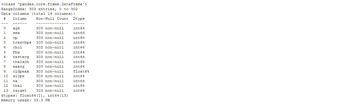
Since we have no missing values and our data does not need any encoding, we can now separate the features from the label.
#X will hold our features and y will hold the label

X = data.drop('target', axis = 1)
y = data['target']
We want to split our data so we can train our model and simulate its performance
#N and D will be housing the data shape

from sklearn.model_selection import train_test_split

X_train, X_test, y_train, y_test = train_test_split(X, y, test_size = 0.2,
                                                    random_state = 42)
N, D = X_train.shape
Next, we scale the data. It is always important to scale your data when using Neural Networks. This helps prevent the model from giving large weights (importance) to features with large values over features with low values.
from sklearn.preprocessing import StandardScaler

scaler = StandardScaler()
X_train = scaler.fit_transform(X_train)
X_test = scaler.transform(X_test)
Next, our model.
model = tf.keras.models.Sequential()
model.add(tf.keras.layers.Dense(1, input_shape=(D,), activation='sigmoid'))

# the model can also be created this way
# reason against doing so in a later cell

# model = tf.keras,models.Sequential
# model.add(tf.keras.layers.Input(shape=(D,)))
# model.add(tf.keras.layers.Dense(1, activation='sigmoid'))
Tensorflow API allows us to specify the input layer in the dense layer which helps with fewer lines of code. We assign sigmoid to the activation parameter because our neural network outputs probabilities for each class/label. The sigmoid function along with a threshold sets these values to be 1 if the probability is more than or equal to the threshold and 0 if it is below the threshold. Note that there are different activation functions
Next, we call the compile method
model.compile(optimizer=tf.keras.optimizers.SGD(lr=0.01, momentum=0.9, decay=0.001),
              loss='binary_crossentropy',
              metrics=['accuracy'],
              )
The optimizer is where we set the type of gradient descent and learning rate. Learning rate is a hyperparameter that controls how much to change the model in response to the estimated error each time the model weights are updated. You always want to test different learning rates to investigate how well your model is performing. Follow this link to understand the dynamics of learning rate.
Since we have only 2 classes/labels, we will be using the binary_crossentropy. When there are more than 2 labels, categorical_crossentropy is used instead. The accuracy metric helps us to know what percentage of our predictions are correct.
It is strongly advised to read the Tensorflow documentation to find the different values that can be set per parameter and their usage.
Next, we want to fit/train our model on the data.
r = model.fit(X_train, y_train, validation_data=(X_test, y_test),
              epochs = 100)
The number of epochs is the number of iteration over the entire dataset. So we want our model to learn on the data 100 times. Again, you want to try different values for your hyperparameters and select the one that works best for you. The validation_data allows us to evaluate our model on data points that were not present in the training process.
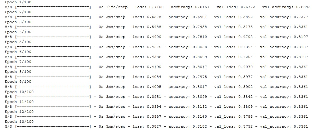
As you see, the loss decreases per iteration. Note that you should reduce the number of epochs at a point where the loss remains the same/increases.
Next, we evaluate our model
print('Train Score: ', model.evaluate(X_train, y_train))
print('Test Score: ', model.evaluate(X_test, y_test))

> 8/8 [==============================] - 0s 1ms/step - loss: 0.3483 - accuracy: 0.8636
> Train Score:  [0.34829163551330566, 0.8636363744735718]
> 2/2 [==============================] - 0s 2ms/step - loss: 0.3685 - accuracy: 0.8525
> Test Score:  [0.36852094531059265, 0.8524590134620667]
This returns the final loss and accuracy. We get an 85% accuracy on the training set and 87% accuracy on the test set... Not bad.
Next, we want to visualise our loss and accuracy. Our model returns a history object where we can access the loss and accuracy.
plt.plot(r.history['loss'], label='loss')
plt.plot(r.history['val_loss'], label='val_loss')
plt.legend()

# If this is running on a local computer, you need to
# enter plt.show() to see the plot
we get
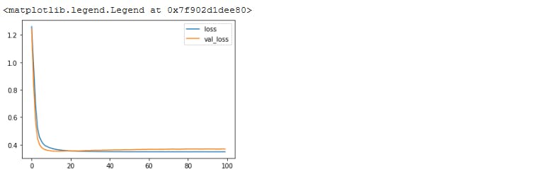
We see that our loss reduces and converges nicely.
Next, we plot our accuracy
plt.plot(r.history['accuracy'], label='acc')
plt.plot(r.history['val_accuracy'], label = 'val_acc')
plt.legend()
we get
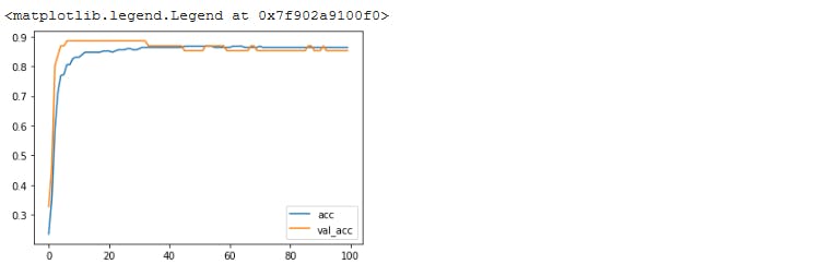
Not bad...
To get predictions on the data, we use the predict method
predictions = model.predict(X_test)
Finally, we save our model
model.save('linearclassifier.h5')
We can load the model and confirm it still works. There is usually a bug in Keras where load/save only works if you do not use the Input() layer explicitly (Check code cell where we set up our layers).
model = tf.keras.models.load_model('linearclassifier.h5')
model.evaluate(X_test, y_test)

> 2/2 [==============================] - 0s 3ms/step - loss: 0.3685 - accuracy: 0.8525

> [0.36852094531059265, 0.8524590134620667]
If you want to download your model from colab to your local computer
from google.colab import files
files.download('linearclassifier.h5')
The filename must match what you set above. You can use the command to download any file from your colab notebook
Summary
We built a Tensorflow model for classification, saved it and loaded it. That makes me feels pretty good. Do you feel good? :)
References and Resources
Get the full code here